Kavi's BGGN 213 Portfolio

Class work for bioinformatics class
Class 10
Kavi Gonur (PID: A69046927)
Importing candy data
candy_file <- read.csv("https://raw.githubusercontent.com/fivethirtyeight/data/master/candy-power-ranking/candy-data.csv")

candy = data.frame(candy_file, row.names=1)
head(candy)
             chocolate fruity caramel peanutyalmondy nougat crispedricewafer
100 Grand            1      0       1              0      0                1
3 Musketeers         1      0       0              0      1                0
One dime             0      0       0              0      0                0
One quarter          0      0       0              0      0                0
Air Heads            0      1       0              0      0                0
Almond Joy           1      0       0              1      0                0
             hard bar pluribus sugarpercent pricepercent winpercent
100 Grand       0   1        0        0.732        0.860   66.97173
3 Musketeers    0   1        0        0.604        0.511   67.60294
One dime        0   0        0        0.011        0.116   32.26109
One quarter     0   0        0        0.011        0.511   46.11650
Air Heads       0   0        0        0.906        0.511   52.34146
Almond Joy      0   1        0        0.465        0.767   50.34755
Q1. How many different candy types are in this dataset?
There are 85 different candy types in the dataset.
Q2. How many fruity candy types are in the dataset?
There are 38 fruity candy types in the dataset.
What is your favorate candy?
Q3. What is your favorite candy in the dataset and what is it’s winpercent value?
I have a ton of favorite candies. How dare you make me choose. ;-; But I suppose right now I like fruitier candy so Haribo Happy Cola. Its winpercent is 34.158958%.
Q4. What is the winpercent value for “Kit Kat”?
76.7686%
Q5. What is the winpercent value for “Tootsie Roll Snack Bars”?
49.653503%
library("skimr")
skim(candy)
| Name | candy |
| Number of rows | 85 |
| Number of columns | 12 |
| _______________________ | |
| Column type frequency: | |
| numeric | 12 |
| ________________________ | |
| Group variables | None |
Data summary
Variable type: numeric
| skim_variable | n_missing | complete_rate | mean | sd | p0 | p25 | p50 | p75 | p100 | hist |
|---|---|---|---|---|---|---|---|---|---|---|
| chocolate | 0 | 1 | 0.44 | 0.50 | 0.00 | 0.00 | 0.00 | 1.00 | 1.00 | ▇▁▁▁▆ |
| fruity | 0 | 1 | 0.45 | 0.50 | 0.00 | 0.00 | 0.00 | 1.00 | 1.00 | ▇▁▁▁▆ |
| caramel | 0 | 1 | 0.16 | 0.37 | 0.00 | 0.00 | 0.00 | 0.00 | 1.00 | ▇▁▁▁▂ |
| peanutyalmondy | 0 | 1 | 0.16 | 0.37 | 0.00 | 0.00 | 0.00 | 0.00 | 1.00 | ▇▁▁▁▂ |
| nougat | 0 | 1 | 0.08 | 0.28 | 0.00 | 0.00 | 0.00 | 0.00 | 1.00 | ▇▁▁▁▁ |
| crispedricewafer | 0 | 1 | 0.08 | 0.28 | 0.00 | 0.00 | 0.00 | 0.00 | 1.00 | ▇▁▁▁▁ |
| hard | 0 | 1 | 0.18 | 0.38 | 0.00 | 0.00 | 0.00 | 0.00 | 1.00 | ▇▁▁▁▂ |
| bar | 0 | 1 | 0.25 | 0.43 | 0.00 | 0.00 | 0.00 | 0.00 | 1.00 | ▇▁▁▁▂ |
| pluribus | 0 | 1 | 0.52 | 0.50 | 0.00 | 0.00 | 1.00 | 1.00 | 1.00 | ▇▁▁▁▇ |
| sugarpercent | 0 | 1 | 0.48 | 0.28 | 0.01 | 0.22 | 0.47 | 0.73 | 0.99 | ▇▇▇▇▆ |
| pricepercent | 0 | 1 | 0.47 | 0.29 | 0.01 | 0.26 | 0.47 | 0.65 | 0.98 | ▇▇▇▇▆ |
| winpercent | 0 | 1 | 50.32 | 14.71 | 22.45 | 39.14 | 47.83 | 59.86 | 84.18 | ▃▇▆▅▂ |
Q6. Is there any variable/column that looks to be on a different scale to the majority of the other columns in the dataset?
Yes. winpercent.
Q7. What do you think a zero and one represent for the candy$chocolate column?
0 = candy is NOT a chocolate. 1 = candy IS a chocolate.
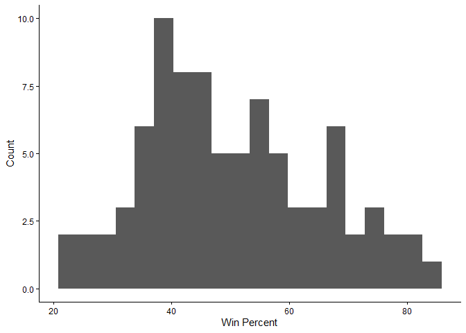
Q8. Plot a histogram of winpercent values
library(ggplot2)
ggplot(candy) +
  aes(x=winpercent) +
  theme_classic() +
  geom_histogram(bins=20) +
  labs(x="Win Percent", y= "Count")
Q9. Is the distribution of winpercent values symmetrical?
ggplot(candy) +
  aes(x=winpercent) +
  theme_classic() +
  geom_density()
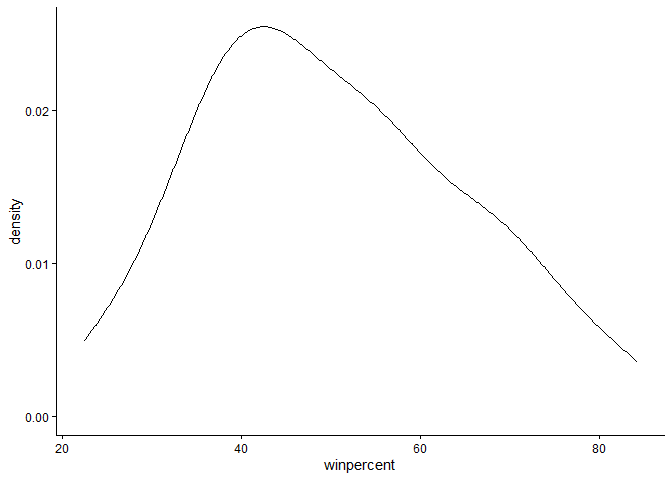
Nope
Q10. Is the center of the distribution above or below 50%?
summary(candy$winpercent)
   Min. 1st Qu.  Median    Mean 3rd Qu.    Max.
  22.45   39.14   47.83   50.32   59.86   84.18
According to the mean, above. But the median is below.
Q11. On average is chocolate candy higher or lower ranked than fruit candy?
# 1. Find all chocolate candy in the dataset
choc.inds <- as.logical(candy$chocolate)
choc.candy <- candy[choc.inds,]
choc.candy
                            chocolate fruity caramel peanutyalmondy nougat
100 Grand                           1      0       1              0      0
3 Musketeers                        1      0       0              0      1
Almond Joy                          1      0       0              1      0
Baby Ruth                           1      0       1              1      1
Charleston Chew                     1      0       0              0      1
Hershey's Kisses                    1      0       0              0      0
Hershey's Krackel                   1      0       0              0      0
Hershey's Milk Chocolate            1      0       0              0      0
Hershey's Special Dark              1      0       0              0      0
Junior Mints                        1      0       0              0      0
Kit Kat                             1      0       0              0      0
Peanut butter M&M's                 1      0       0              1      0
M&M's                               1      0       0              0      0
Milk Duds                           1      0       1              0      0
Milky Way                           1      0       1              0      1
Milky Way Midnight                  1      0       1              0      1
Milky Way Simply Caramel            1      0       1              0      0
Mounds                              1      0       0              0      0
Mr Good Bar                         1      0       0              1      0
Nestle Butterfinger                 1      0       0              1      0
Nestle Crunch                       1      0       0              0      0
Peanut M&Ms                         1      0       0              1      0
Reese's Miniatures                  1      0       0              1      0
Reese's Peanut Butter cup           1      0       0              1      0
Reese's pieces                      1      0       0              1      0
Reese's stuffed with pieces         1      0       0              1      0
Rolo                                1      0       1              0      0
Sixlets                             1      0       0              0      0
Nestle Smarties                     1      0       0              0      0
Snickers                            1      0       1              1      1
Snickers Crisper                    1      0       1              1      0
Tootsie Pop                         1      1       0              0      0
Tootsie Roll Juniors                1      0       0              0      0
Tootsie Roll Midgies                1      0       0              0      0
Tootsie Roll Snack Bars             1      0       0              0      0
Twix                                1      0       1              0      0
Whoppers                            1      0       0              0      0
                            crispedricewafer hard bar pluribus sugarpercent
100 Grand                                  1    0   1        0        0.732
3 Musketeers                               0    0   1        0        0.604
Almond Joy                                 0    0   1        0        0.465
Baby Ruth                                  0    0   1        0        0.604
Charleston Chew                            0    0   1        0        0.604
Hershey's Kisses                           0    0   0        1        0.127
Hershey's Krackel                          1    0   1        0        0.430
Hershey's Milk Chocolate                   0    0   1        0        0.430
Hershey's Special Dark                     0    0   1        0        0.430
Junior Mints                               0    0   0        1        0.197
Kit Kat                                    1    0   1        0        0.313
Peanut butter M&M's                        0    0   0        1        0.825
M&M's                                      0    0   0        1        0.825
Milk Duds                                  0    0   0        1        0.302
Milky Way                                  0    0   1        0        0.604
Milky Way Midnight                         0    0   1        0        0.732
Milky Way Simply Caramel                   0    0   1        0        0.965
Mounds                                     0    0   1        0        0.313
Mr Good Bar                                0    0   1        0        0.313
Nestle Butterfinger                        0    0   1        0        0.604
Nestle Crunch                              1    0   1        0        0.313
Peanut M&Ms                                0    0   0        1        0.593
Reese's Miniatures                         0    0   0        0        0.034
Reese's Peanut Butter cup                  0    0   0        0        0.720
Reese's pieces                             0    0   0        1        0.406
Reese's stuffed with pieces                0    0   0        0        0.988
Rolo                                       0    0   0        1        0.860
Sixlets                                    0    0   0        1        0.220
Nestle Smarties                            0    0   0        1        0.267
Snickers                                   0    0   1        0        0.546
Snickers Crisper                           1    0   1        0        0.604
Tootsie Pop                                0    1   0        0        0.604
Tootsie Roll Juniors                       0    0   0        0        0.313
Tootsie Roll Midgies                       0    0   0        1        0.174
Tootsie Roll Snack Bars                    0    0   1        0        0.465
Twix                                       1    0   1        0        0.546
Whoppers                                   1    0   0        1        0.872
                            pricepercent winpercent
100 Grand                          0.860   66.97173
3 Musketeers                       0.511   67.60294
Almond Joy                         0.767   50.34755
Baby Ruth                          0.767   56.91455
Charleston Chew                    0.511   38.97504
Hershey's Kisses                   0.093   55.37545
Hershey's Krackel                  0.918   62.28448
Hershey's Milk Chocolate           0.918   56.49050
Hershey's Special Dark             0.918   59.23612
Junior Mints                       0.511   57.21925
Kit Kat                            0.511   76.76860
Peanut butter M&M's                0.651   71.46505
M&M's                              0.651   66.57458
Milk Duds                          0.511   55.06407
Milky Way                          0.651   73.09956
Milky Way Midnight                 0.441   60.80070
Milky Way Simply Caramel           0.860   64.35334
Mounds                             0.860   47.82975
Mr Good Bar                        0.918   54.52645
Nestle Butterfinger                0.767   70.73564
Nestle Crunch                      0.767   66.47068
Peanut M&Ms                        0.651   69.48379
Reese's Miniatures                 0.279   81.86626
Reese's Peanut Butter cup          0.651   84.18029
Reese's pieces                     0.651   73.43499
Reese's stuffed with pieces        0.651   72.88790
Rolo                               0.860   65.71629
Sixlets                            0.081   34.72200
Nestle Smarties                    0.976   37.88719
Snickers                           0.651   76.67378
Snickers Crisper                   0.651   59.52925
Tootsie Pop                        0.325   48.98265
Tootsie Roll Juniors               0.511   43.06890
Tootsie Roll Midgies               0.011   45.73675
Tootsie Roll Snack Bars            0.325   49.65350
Twix                               0.906   81.64291
Whoppers                           0.848   49.52411
# 2. Extract their `winpercent` values
choc.win <- choc.candy$winpercent

# 3. Find the mean of these values
choc.mean <- mean(choc.win)

# 4-6. Do the same for fruity candy
fruity.inds <- as.logical(candy$fruity)
fruity.candy <- candy[fruity.inds,]
fruity.win <- fruity.candy$winpercent
fruity.mean <- mean(fruity.win)
fruity.mean
[1] 44.11974
# 7. Which mean value is higher?
if (fruity.mean > choc.mean) {
  print("Fruity")
} else {
  print("Chocolate")
}
[1] "Chocolate"
Q12. Is this difference statistically significant?
t.test(choc.win,fruity.win)
    Welch Two Sample t-test

data:  choc.win and fruity.win
t = 6.2582, df = 68.882, p-value = 2.871e-08
alternative hypothesis: true difference in means is not equal to 0
95 percent confidence interval:
 11.44563 22.15795
sample estimates:
mean of x mean of y
 60.92153  44.11974
Overall Candy Rankings
Q13. What are the five least liked candy types in this set?
library(dplyr)
Attaching package: 'dplyr'

The following objects are masked from 'package:stats':

    filter, lag

The following objects are masked from 'package:base':

    intersect, setdiff, setequal, union
candy %>%
arrange(winpercent) %>%
head(5)
                   chocolate fruity caramel peanutyalmondy nougat
Nik L Nip                  0      1       0              0      0
Boston Baked Beans         0      0       0              1      0
Chiclets                   0      1       0              0      0
Super Bubble               0      1       0              0      0
Jawbusters                 0      1       0              0      0
                   crispedricewafer hard bar pluribus sugarpercent pricepercent
Nik L Nip                         0    0   0        1        0.197        0.976
Boston Baked Beans                0    0   0        1        0.313        0.511
Chiclets                          0    0   0        1        0.046        0.325
Super Bubble                      0    0   0        0        0.162        0.116
Jawbusters                        0    1   0        1        0.093        0.511
                   winpercent
Nik L Nip            22.44534
Boston Baked Beans   23.41782
Chiclets             24.52499
Super Bubble         27.30386
Jawbusters           28.12744
Q14. What are the top 5 all time favorite candy types out of this set?
library(dplyr)
candy %>%
arrange(winpercent) %>%
tail(5)
                          chocolate fruity caramel peanutyalmondy nougat
Snickers                          1      0       1              1      1
Kit Kat                           1      0       0              0      0
Twix                              1      0       1              0      0
Reese's Miniatures                1      0       0              1      0
Reese's Peanut Butter cup         1      0       0              1      0
                          crispedricewafer hard bar pluribus sugarpercent
Snickers                                 0    0   1        0        0.546
Kit Kat                                  1    0   1        0        0.313
Twix                                     1    0   1        0        0.546
Reese's Miniatures                       0    0   0        0        0.034
Reese's Peanut Butter cup                0    0   0        0        0.720
                          pricepercent winpercent
Snickers                         0.651   76.67378
Kit Kat                          0.511   76.76860
Twix                             0.906   81.64291
Reese's Miniatures               0.279   81.86626
Reese's Peanut Butter cup        0.651   84.18029
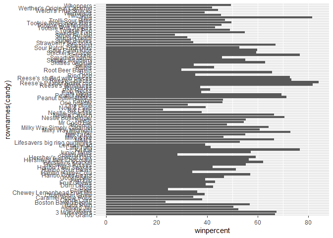
Q15. Make a first barplot of candy ranking based on winpercent values.
library(ggplot2)
ggplot(candy) +
  aes(winpercent, rownames(candy)) +
  geom_col()
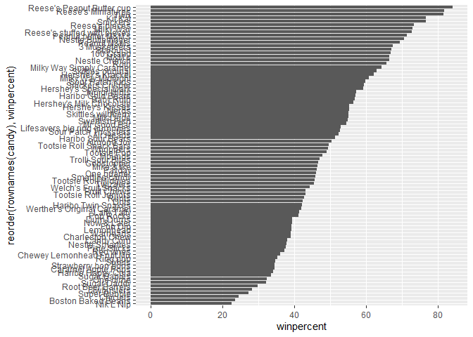
Q16. This is quite ugly, use the reorder() function to get the bars sorted by winpercent?
ggplot(candy) +
  aes(winpercent, reorder(rownames(candy),winpercent)) +
  geom_col()
Time to add some useful color
my_cols=rep("black", nrow(candy))
my_cols[as.logical(candy$chocolate)] = "chocolate"
my_cols[as.logical(candy$bar)] = "brown"
my_cols[as.logical(candy$fruity)] = "pink"

ggplot(candy) +
  aes(winpercent, reorder(rownames(candy),winpercent)) +
  geom_col(fill=my_cols)
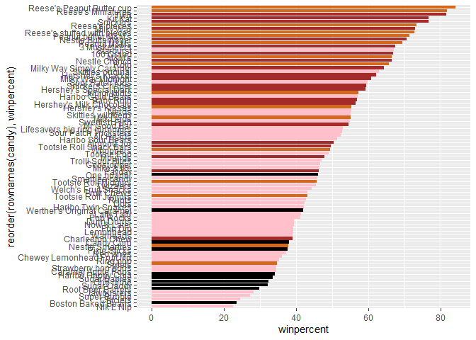
Q17. What is the worst ranked chocolate candy?
Sixlets
Q18. What is the best ranked fruity candy?
Starburst
Taking a look at pricepercent
library(ggrepel)

# How about a plot of price vs win
ggplot(candy) +
  aes(winpercent, pricepercent, label=rownames(candy)) +
  geom_point(col=my_cols) +
  geom_text_repel(col=my_cols, size=3.3, max.overlaps = 5)
Warning: ggrepel: 54 unlabeled data points (too many overlaps). Consider
increasing max.overlaps
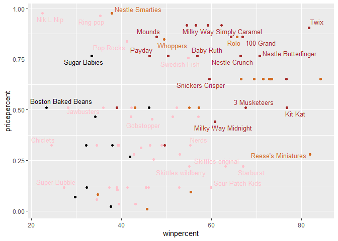
Q19. Which candy type is the highest ranked in terms of winpercent for the least money - i.e. offers the most bang for your buck?
ord <- order(candy$pricepercent, decreasing = FALSE)
head( candy[ord,c("pricepercent", "winpercent")], n=5 )
                     pricepercent winpercent
Tootsie Roll Midgies        0.011   45.73675
Pixie Sticks                0.023   37.72234
Dum Dums                    0.034   39.46056
Fruit Chews                 0.034   43.08892
Strawberry bon bons         0.058   34.57899
Tootsie Roll Midgies
Q20. What are the top 5 most expensive candy types in the dataset and of these which is the least popular?
ord <- order(candy$pricepercent, decreasing = TRUE)
head( candy[ord,c("pricepercent", "winpercent")], n=5 )
                         pricepercent winpercent
Nik L Nip                       0.976   22.44534
Nestle Smarties                 0.976   37.88719
Ring pop                        0.965   35.29076
Hershey's Krackel               0.918   62.28448
Hershey's Milk Chocolate        0.918   56.49050
Nik L Nips
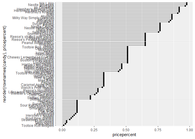
Q21. Make a barplot again with geom_col() this time using pricepercent and then improve this step by step, first ordering the x-axis by value and finally making a so called “dot chat” or “lollipop” chart by swapping geom_col() for geom_point() + geom_segment()
ggplot(candy) +
  aes(pricepercent, reorder(rownames(candy), pricepercent)) +
  geom_segment(aes(yend = reorder(rownames(candy), pricepercent),
                   xend = 0), col="gray40") +
    geom_point()
Exploring the correlation structure
library(corrplot)
corrplot 0.95 loaded
cij <- cor(candy)
cij
                  chocolate      fruity     caramel peanutyalmondy      nougat
chocolate         1.0000000 -0.74172106  0.24987535     0.37782357  0.25489183
fruity           -0.7417211  1.00000000 -0.33548538    -0.39928014 -0.26936712
caramel           0.2498753 -0.33548538  1.00000000     0.05935614  0.32849280
peanutyalmondy    0.3778236 -0.39928014  0.05935614     1.00000000  0.21311310
nougat            0.2548918 -0.26936712  0.32849280     0.21311310  1.00000000
crispedricewafer  0.3412098 -0.26936712  0.21311310    -0.01764631 -0.08974359
hard             -0.3441769  0.39067750 -0.12235513    -0.20555661 -0.13867505
bar               0.5974211 -0.51506558  0.33396002     0.26041960  0.52297636
pluribus         -0.3396752  0.29972522 -0.26958501    -0.20610932 -0.31033884
sugarpercent      0.1041691 -0.03439296  0.22193335     0.08788927  0.12308135
pricepercent      0.5046754 -0.43096853  0.25432709     0.30915323  0.15319643
winpercent        0.6365167 -0.38093814  0.21341630     0.40619220  0.19937530
                 crispedricewafer        hard         bar    pluribus
chocolate              0.34120978 -0.34417691  0.59742114 -0.33967519
fruity                -0.26936712  0.39067750 -0.51506558  0.29972522
caramel                0.21311310 -0.12235513  0.33396002 -0.26958501
peanutyalmondy        -0.01764631 -0.20555661  0.26041960 -0.20610932
nougat                -0.08974359 -0.13867505  0.52297636 -0.31033884
crispedricewafer       1.00000000 -0.13867505  0.42375093 -0.22469338
hard                  -0.13867505  1.00000000 -0.26516504  0.01453172
bar                    0.42375093 -0.26516504  1.00000000 -0.59340892
pluribus              -0.22469338  0.01453172 -0.59340892  1.00000000
sugarpercent           0.06994969  0.09180975  0.09998516  0.04552282
pricepercent           0.32826539 -0.24436534  0.51840654 -0.22079363
winpercent             0.32467965 -0.31038158  0.42992933 -0.24744787
                 sugarpercent pricepercent winpercent
chocolate          0.10416906    0.5046754  0.6365167
fruity            -0.03439296   -0.4309685 -0.3809381
caramel            0.22193335    0.2543271  0.2134163
peanutyalmondy     0.08788927    0.3091532  0.4061922
nougat             0.12308135    0.1531964  0.1993753
crispedricewafer   0.06994969    0.3282654  0.3246797
hard               0.09180975   -0.2443653 -0.3103816
bar                0.09998516    0.5184065  0.4299293
pluribus           0.04552282   -0.2207936 -0.2474479
sugarpercent       1.00000000    0.3297064  0.2291507
pricepercent       0.32970639    1.0000000  0.3453254
winpercent         0.22915066    0.3453254  1.0000000
corrplot(cij)
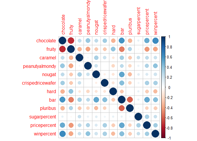
Q22. Examining this plot what two variables are anti-correlated (i.e. have minus values)?
- Fruity + chocolate/caramel/peanutyalmondy/nougat/crispedricewafer/bar
Q23. Similarly, what two variables are most positively correlated?
- chocolate + bar or chocolate + winpercent
Principal Component Analysis
pca <- prcomp(candy, scale=TRUE)
summary(pca)
Importance of components:
                          PC1    PC2    PC3     PC4    PC5     PC6     PC7
Standard deviation     2.0788 1.1378 1.1092 1.07533 0.9518 0.81923 0.81530
Proportion of Variance 0.3601 0.1079 0.1025 0.09636 0.0755 0.05593 0.05539
Cumulative Proportion  0.3601 0.4680 0.5705 0.66688 0.7424 0.79830 0.85369
                           PC8     PC9    PC10    PC11    PC12
Standard deviation     0.74530 0.67824 0.62349 0.43974 0.39760
Proportion of Variance 0.04629 0.03833 0.03239 0.01611 0.01317
Cumulative Proportion  0.89998 0.93832 0.97071 0.98683 1.00000
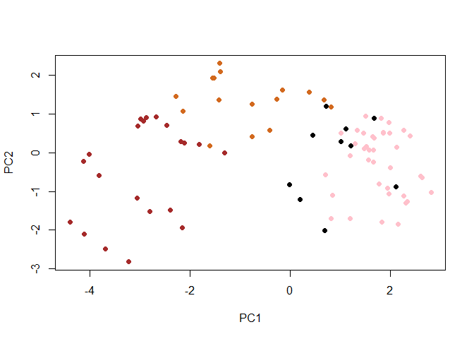
plot(pca$x[,1:2], col=my_cols, pch=16)
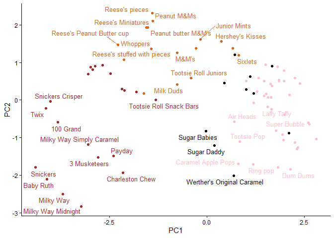
ggplot(pca$x) +
  aes(PC1,PC2) +
  geom_point(col=my_cols) +
  theme_classic() +
  geom_text_repel(aes(label = rownames(pca$x)), color = my_cols, size = 3.3, max.overlaps = 5)
Warning: ggrepel: 50 unlabeled data points (too many overlaps). Consider
increasing max.overlaps
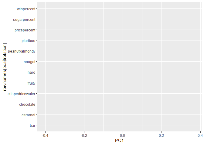
ggplot(pca$rotation) +
  aes(PC1,rownames(pca$rotation))
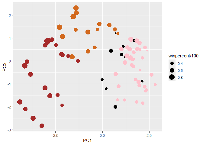
my_data <- cbind(candy, pca$x[,1:3])
p <- ggplot(my_data) +
        aes(x=PC1, y=PC2,
            size=winpercent/100,
            text=rownames(my_data),
            label=rownames(my_data)) +
        geom_point(col=my_cols)

p