Kavi's BGGN 213 Portfolio

Class work for bioinformatics class
Class 12
Kavi (PID: )
- Background
- Data Import
- Toy analysis example
- DESeq Analysis
- Volcano Plot
- Save our results
- Pathway Analysis
- Adḍ annotation data
- Save my annotated results
Background
Today we will analyze some RNASeq data from Himes et al. on the effectṡof a common steroid (dexamethasone, also called “dex”) on ariway smooth muscle cells (ASMs).
For this analysis we need two main inputs
countData: a table of counts per gene (in rows) across experiments (in columns)colData: metadata about the design of the experiments. The rows here must match the columns incountData
Data Import
counts <- read.csv("airway_scaledcounts.csv", row.names=1)
metadata <-  read.csv("airway_metadata.csv")
head(counts)
                SRR1039508 SRR1039509 SRR1039512 SRR1039513 SRR1039516
ENSG00000000003        723        486        904        445       1170
ENSG00000000005          0          0          0          0          0
ENSG00000000419        467        523        616        371        582
ENSG00000000457        347        258        364        237        318
ENSG00000000460         96         81         73         66        118
ENSG00000000938          0          0          1          0          2
                SRR1039517 SRR1039520 SRR1039521
ENSG00000000003       1097        806        604
ENSG00000000005          0          0          0
ENSG00000000419        781        417        509
ENSG00000000457        447        330        324
ENSG00000000460         94        102         74
ENSG00000000938          0          0          0
and the metadata:
metadata
          id     dex celltype     geo_id
1 SRR1039508 control   N61311 GSM1275862
2 SRR1039509 treated   N61311 GSM1275863
3 SRR1039512 control  N052611 GSM1275866
4 SRR1039513 treated  N052611 GSM1275867
5 SRR1039516 control  N080611 GSM1275870
6 SRR1039517 treated  N080611 GSM1275871
7 SRR1039520 control  N061011 GSM1275874
8 SRR1039521 treated  N061011 GSM1275875
Q1. How many “genes” are in this dataset?
There are 38694 genes in the dataset.
Q2. How many experiments (i.e. columns in
countsor rows inmetadata) are there?
If we use counts: 8
If we use metadata: 8
Q3. How many “control” experiments are there in the dataset?
There are 4 “control” experiments.
Toy analysis example
Contains answers to Q3 and Q4.
- Extract the “control” columns from
counts. - Calculate the mean value for each gene in these “control” columns.
3-4. Do the same for the “treated” columns. 5. Compare these mean values for each gene.
Step 1
control.inds <- metadata$dex == "control"
control.counts <- counts[, control.inds]
head(control.counts)
                SRR1039508 SRR1039512 SRR1039516 SRR1039520
ENSG00000000003        723        904       1170        806
ENSG00000000005          0          0          0          0
ENSG00000000419        467        616        582        417
ENSG00000000457        347        364        318        330
ENSG00000000460         96         73        118        102
ENSG00000000938          0          1          2          0
Step 2
control.mean <- rowMeans(control.counts)
Steps 3-4
treated.inds <- metadata$dex == "treated"
treated.counts <- counts[, treated.inds]
head(treated.counts)
                SRR1039509 SRR1039513 SRR1039517 SRR1039521
ENSG00000000003        486        445       1097        604
ENSG00000000005          0          0          0          0
ENSG00000000419        523        371        781        509
ENSG00000000457        258        237        447        324
ENSG00000000460         81         66         94         74
ENSG00000000938          0          0          0          0
treated.mean <- rowMeans(treated.counts)
For ease of book-keeping we can store these together in one data frame
called meancounts
meancounts <- data.frame(control.mean,treated.mean)
head(meancounts)
                control.mean treated.mean
ENSG00000000003       900.75       658.00
ENSG00000000005         0.00         0.00
ENSG00000000419       520.50       546.00
ENSG00000000457       339.75       316.50
ENSG00000000460        97.25        78.75
ENSG00000000938         0.75         0.00
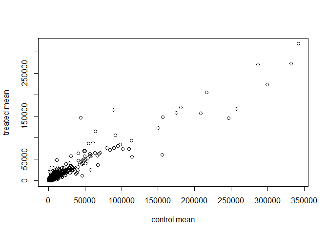
Step 5 > These are answers to Q5 a and b.
plot(control.mean, treated.mean)
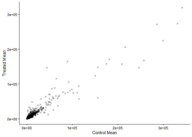
library(ggplot2)
ggplot(meancounts) +
  aes(x=control.mean,y=treated.mean) +
  labs(x="Control Mean", y="Treated Mean") +
  geom_point(alpha=0.2) +
  theme_classic()
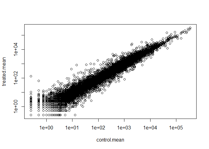
This is the answer to Q6.
plot(control.mean, treated.mean,log="xy")
Warning in xy.coords(x, y, xlabel, ylabel, log): 15032 x values <= 0 omitted
from logarithmic plot

Warning in xy.coords(x, y, xlabel, ylabel, log): 15281 y values <= 0 omitted
from logarithmic plot
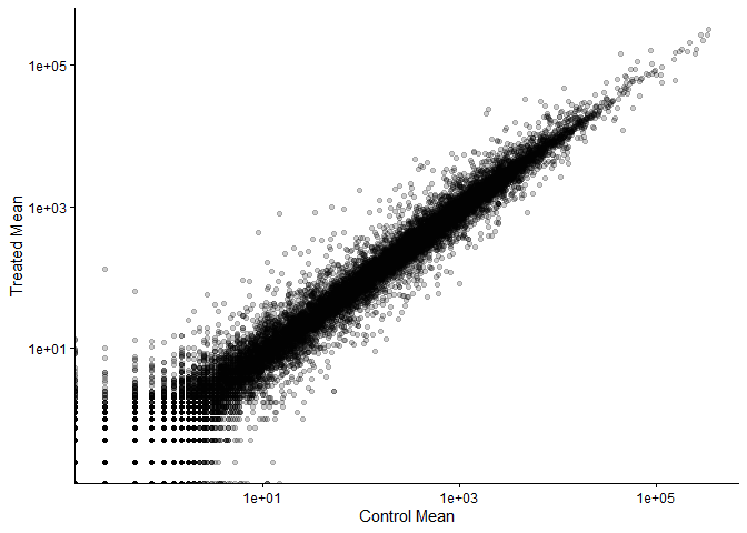
ggplot(meancounts) +
  aes(x=control.mean,y=treated.mean) +
  labs(x="Control Mean", y="Treated Mean") +
  geom_point(alpha=0.2) +
  scale_x_log10() +
  scale_y_log10() +
  theme_classic()
Warning in scale_x_log10(): log-10 transformation introduced infinite values.

Warning in scale_y_log10(): log-10 transformation introduced infinite values.
We use “fold-change” as a way to compare
log2(10/10)
[1] 0
log2(20/10)
[1] 1
log2(10/20)
[1] -1
log2(40/10)
[1] 2
meancounts$log2fc <- log2(meancounts$treated.mean/meancounts$control.mean)
head(meancounts)
                control.mean treated.mean      log2fc
ENSG00000000003       900.75       658.00 -0.45303916
ENSG00000000005         0.00         0.00         NaN
ENSG00000000419       520.50       546.00  0.06900279
ENSG00000000457       339.75       316.50 -0.10226805
ENSG00000000460        97.25        78.75 -0.30441833
ENSG00000000938         0.75         0.00        -Inf
zero.vals <- which(meancounts[,1:2]==0, arr.ind=TRUE)

to.rm <- unique(zero.vals[,1])
mycounts <- meancounts[-to.rm,]
head(mycounts)
                control.mean treated.mean      log2fc
ENSG00000000003       900.75       658.00 -0.45303916
ENSG00000000419       520.50       546.00  0.06900279
ENSG00000000457       339.75       316.50 -0.10226805
ENSG00000000460        97.25        78.75 -0.30441833
ENSG00000000971      5219.00      6687.50  0.35769358
ENSG00000001036      2327.00      1785.75 -0.38194109
A common “rule of thumb” threshold for calling something “up” regulated is a log2-fold-change of +2 or greater. For “down” regulated, a log2-fold-change of -2 or lower.
Q8 How many genes are “up” regulated at the +2 log2FC threshold?
nonzero.inds <- rowSums(counts) != 0
mycounts <- meancounts[nonzero.inds,]
sum(mycounts$log2fc >= 2)
[1] 1910
sum(meancounts$log2fc >= 2, na.rm = T)
[1] 1910
zero.inds <- which(meancounts[,1:2]==0,arr.ind=T)[,1]
mygenes <- meancounts[-zero.inds,]
sum(mygenes$log2fc >= 2)
[1] 314
How many genes are “down” regulated (at the -2 log2FC threshold)?
nonzero.inds <- rowSums(counts) != 0
mycounts <- meancounts[nonzero.inds,]
sum(mycounts$log2fc <= -2)
[1] 2330
sum(meancounts$log2fc <= -2, na.rm = T)
[1] 2330
zero.inds <- which(meancounts[,1:2]==0,arr.ind=T)[,1]
mygenes <- meancounts[-zero.inds,]
sum(mygenes$log2fc <= -2)
[1] 485
DESeq Analysis
Let’s do this with DESeq2 and put some stats behind these numbers
library(DESeq2)
Warning: package 'matrixStats' was built under R version 4.5.2
DESeq wants 3 things for analysis, countData, colData, and design.
dds <- DESeqDataSetFromMatrix(countData =counts,
                       colData = metadata,
                       design = ~dex)
converting counts to integer mode

Warning in DESeqDataSet(se, design = design, ignoreRank): some variables in
design formula are characters, converting to factors
The main function in the DESeq package to run analysis is called
DESeq().
dds <- DESeq(dds)
estimating size factors

estimating dispersions

gene-wise dispersion estimates

mean-dispersion relationship

final dispersion estimates

fitting model and testing
Get the results out of this DESeq object with the function results().
res <- results(dds)
head(res)
log2 fold change (MLE): dex treated vs control
Wald test p-value: dex treated vs control
DataFrame with 6 rows and 6 columns
                  baseMean log2FoldChange     lfcSE      stat    pvalue
                 <numeric>      <numeric> <numeric> <numeric> <numeric>
ENSG00000000003 747.194195     -0.3507030  0.168246 -2.084470 0.0371175
ENSG00000000005   0.000000             NA        NA        NA        NA
ENSG00000000419 520.134160      0.2061078  0.101059  2.039475 0.0414026
ENSG00000000457 322.664844      0.0245269  0.145145  0.168982 0.8658106
ENSG00000000460  87.682625     -0.1471420  0.257007 -0.572521 0.5669691
ENSG00000000938   0.319167     -1.7322890  3.493601 -0.495846 0.6200029
                     padj
                <numeric>
ENSG00000000003  0.163035
ENSG00000000005        NA
ENSG00000000419  0.176032
ENSG00000000457  0.961694
ENSG00000000460  0.815849
ENSG00000000938        NA
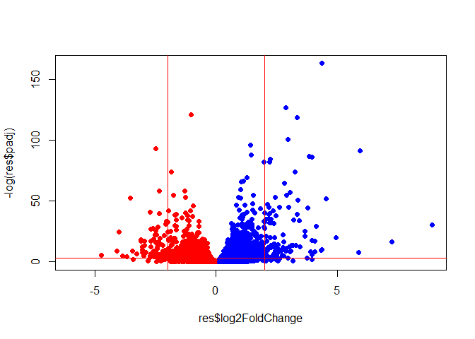
Volcano Plot
This is a plot of log2FC vs adjusted p-value
colors <- ifelse(res$log2FoldChange > 0, "blue", "red")
plot(res$log2FoldChange, -log(res$padj), col = colors, pch = 16)
abline(v = c(-2, 2), col = "red")
abline(h = -log(0.05), col = "red")
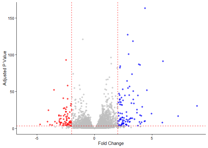
mycols <- rep("gray", nrow(res))               # Start with gray for all
mycols[res$log2FoldChange >= 2] <- "blue"     # Positive large fold changes blue
mycols[res$log2FoldChange <= -2] <- "red"     # Negative large fold changes red
mycols[res$padj >= 0.05] <- "gray"            # Non-significant grey regardless


ggplot(res) +
  aes(x = log2FoldChange, y = -log(padj)) +
  geom_point(color = mycols, alpha = 0.6) +
  theme_classic() +
  geom_vline(xintercept = c(-2, 2), color = "red", linetype = "dashed") +
  geom_hline(yintercept = -log(0.05), color = "red", linetype = "dashed") +
  labs(x = "Fold Change", y = "Adjusted P Value")
Warning: Removed 23549 rows containing missing values or values outside the scale range
(`geom_point()`).
Save our results
write.csv(res,file="BGGN213_Class12Results.csv")
Pathway Analysis
library(pathview)
##############################################################################
Pathview is an open source software package distributed under GNU General
Public License version 3 (GPLv3). Details of GPLv3 is available at
http://www.gnu.org/licenses/gpl-3.0.html. Particullary, users are required to
formally cite the original Pathview paper (not just mention it) in publications
or products. For details, do citation("pathview") within R.

The pathview downloads and uses KEGG data. Non-academic uses may require a KEGG
license agreement (details at http://www.kegg.jp/kegg/legal.html).
##############################################################################
library(gage)
library(gageData)

data(kegg.sets.hs)

# Examine the first 2 pathways in this kegg set for humans
head(kegg.sets.hs, 2)
$`hsa00232 Caffeine metabolism`
[1] "10"   "1544" "1548" "1549" "1553" "7498" "9"

$`hsa00983 Drug metabolism - other enzymes`
 [1] "10"     "1066"   "10720"  "10941"  "151531" "1548"   "1549"   "1551"
 [9] "1553"   "1576"   "1577"   "1806"   "1807"   "1890"   "221223" "2990"
[17] "3251"   "3614"   "3615"   "3704"   "51733"  "54490"  "54575"  "54576"
[25] "54577"  "54578"  "54579"  "54600"  "54657"  "54658"  "54659"  "54963"
[33] "574537" "64816"  "7083"   "7084"   "7172"   "7363"   "7364"   "7365"
[41] "7366"   "7367"   "7371"   "7372"   "7378"   "7498"   "79799"  "83549"
[49] "8824"   "8833"   "9"      "978"
foldchanges = res$log2FoldChange
names(foldchanges) = res$entrez
head(foldchanges)
[1] -0.35070302 NA 0.20610777 0.02452695 -0.14714205 -1.73228897
# Get the results
keggres = gage(foldchanges, gsets=kegg.sets.hs)

attributes(keggres)
$names
[1] "greater" "less"    "stats"
# Look at the first three down (less) pathways
head(keggres$less, 3)
                                         p.geomean stat.mean p.val q.val
hsa00232 Caffeine metabolism                    NA       NaN    NA    NA
hsa00983 Drug metabolism - other enzymes        NA       NaN    NA    NA
hsa01100 Metabolic pathways                     NA       NaN    NA    NA
                                         set.size exp1
hsa00232 Caffeine metabolism                    0   NA
hsa00983 Drug metabolism - other enzymes        0   NA
hsa01100 Metabolic pathways                     0   NA
pathview(gene.data=foldchanges, pathway.id="hsa05310")
Warning: None of the genes or compounds mapped to the pathway!
Argument gene.idtype or cpd.idtype may be wrong.

'select()' returned 1:1 mapping between keys and columns

Info: Working in directory C:/Users/kavan/Desktop/bggn213_f25_github/Class 12

Info: Writing image file hsa05310.pathview.png
 We will use the gage function from
Bioconductor.
We will use the gage function from
Bioconductor.
What gage wants as an inpiy is a simple named vector of importance (i.e. a vector with labeled fold changes)
library(gage)
library(gageData)
foldchanges <- res$log2FoldChange
names(foldchanges) <- res$entrezid
head(foldchanges)
[1] -0.35070302 NA 0.20610777 0.02452695 -0.14714205 -1.73228897
data(kegg.sets.hs)
keggres = gage(foldchanges, gsets=kegg.sets.hs)
head(keggres$less,5)
                                         p.geomean stat.mean p.val q.val
hsa00232 Caffeine metabolism                    NA       NaN    NA    NA
hsa00983 Drug metabolism - other enzymes        NA       NaN    NA    NA
hsa01100 Metabolic pathways                     NA       NaN    NA    NA
hsa00230 Purine metabolism                      NA       NaN    NA    NA
hsa05340 Primary immunodeficiency               NA       NaN    NA    NA
                                         set.size exp1
hsa00232 Caffeine metabolism                    0   NA
hsa00983 Drug metabolism - other enzymes        0   NA
hsa01100 Metabolic pathways                     0   NA
hsa00230 Purine metabolism                      0   NA
hsa05340 Primary immunodeficiency               0   NA
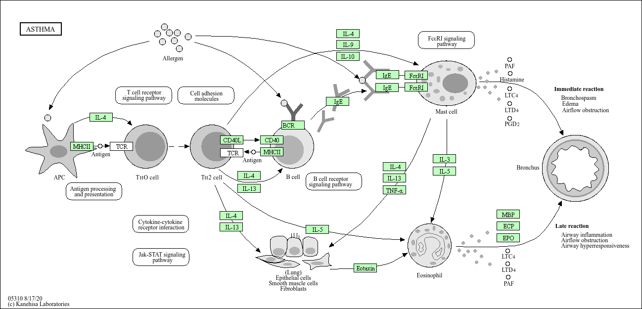
Let’s take a look at just one of these hsa05310
library(pathview)
pathview(gene.data=foldchanges, pathway.id="hsa05310")
Warning: None of the genes or compounds mapped to the pathway!
Argument gene.idtype or cpd.idtype may be wrong.

'select()' returned 1:1 mapping between keys and columns

Info: Working in directory C:/Users/kavan/Desktop/bggn213_f25_github/Class 12

Info: Writing image file hsa05310.pathview.png
Adḍ annotation data
We need to add gene symbols, gene names, and other database ids to make my results useful for future analyses.
head(res)
log2 fold change (MLE): dex treated vs control
Wald test p-value: dex treated vs control
DataFrame with 6 rows and 6 columns
                  baseMean log2FoldChange     lfcSE      stat    pvalue
                 <numeric>      <numeric> <numeric> <numeric> <numeric>
ENSG00000000003 747.194195     -0.3507030  0.168246 -2.084470 0.0371175
ENSG00000000005   0.000000             NA        NA        NA        NA
ENSG00000000419 520.134160      0.2061078  0.101059  2.039475 0.0414026
ENSG00000000457 322.664844      0.0245269  0.145145  0.168982 0.8658106
ENSG00000000460  87.682625     -0.1471420  0.257007 -0.572521 0.5669691
ENSG00000000938   0.319167     -1.7322890  3.493601 -0.495846 0.6200029
                     padj
                <numeric>
ENSG00000000003  0.163035
ENSG00000000005        NA
ENSG00000000419  0.176032
ENSG00000000457  0.961694
ENSG00000000460  0.815849
ENSG00000000938        NA
We have ENSEMBLE database IDs in our res object
head(rownames(res))
[1] "ENSG00000000003" "ENSG00000000005" "ENSG00000000419" "ENSG00000000457"
[5] "ENSG00000000460" "ENSG00000000938"
We can use the mapIDs() function from Bioconductor to help us:
library("AnnotationDbi")
library("org.Hs.eg.db")
Let’s see what database ID formats we can translate into
columns(org.Hs.eg.db)
 [1] "ACCNUM"       "ALIAS"        "ENSEMBL"      "ENSEMBLPROT"  "ENSEMBLTRANS"
 [6] "ENTREZID"     "ENZYME"       "EVIDENCE"     "EVIDENCEALL"  "GENENAME"
[11] "GENETYPE"     "GO"           "GOALL"        "IPI"          "MAP"
[16] "OMIM"         "ONTOLOGY"     "ONTOLOGYALL"  "PATH"         "PFAM"
[21] "PMID"         "PROSITE"      "REFSEQ"       "SYMBOL"       "UCSCKG"
[26] "UNIPROT"
res$symbol <- mapIds(org.Hs.eg.db,
                     keys=row.names(res), # Our genenames
                     keytype="ENSEMBL",        # The format of our genenames
                     column="SYMBOL",          # The new format we want to add
                     multiVals="first")
'select()' returned 1:many mapping between keys and columns
head(res$symbol)
ENSG00000000003 ENSG00000000005 ENSG00000000419 ENSG00000000457 ENSG00000000460
       "TSPAN6"          "TNMD"          "DPM1"         "SCYL3"         "FIRRM"
ENSG00000000938
          "FGR"
Add GENENAME then ENTREZID
res$genename <- mapIds(org.Hs.eg.db,
                     keys=row.names(res), # Our genenames
                     keytype="ENSEMBL",        # The format of our genenames
                     column="GENENAME",          # The new format we want to add
                     multiVals="first")
'select()' returned 1:many mapping between keys and columns
res$entrezid <- mapIds(org.Hs.eg.db,
                     keys=row.names(res), # Our genenames
                     keytype="ENSEMBL",        # The format of our genenames
                     column="ENTREZID",          # The new format we want to add
                     multiVals="first")
'select()' returned 1:many mapping between keys and columns
head(res)
log2 fold change (MLE): dex treated vs control
Wald test p-value: dex treated vs control
DataFrame with 6 rows and 9 columns
                  baseMean log2FoldChange     lfcSE      stat    pvalue
                 <numeric>      <numeric> <numeric> <numeric> <numeric>
ENSG00000000003 747.194195     -0.3507030  0.168246 -2.084470 0.0371175
ENSG00000000005   0.000000             NA        NA        NA        NA
ENSG00000000419 520.134160      0.2061078  0.101059  2.039475 0.0414026
ENSG00000000457 322.664844      0.0245269  0.145145  0.168982 0.8658106
ENSG00000000460  87.682625     -0.1471420  0.257007 -0.572521 0.5669691
ENSG00000000938   0.319167     -1.7322890  3.493601 -0.495846 0.6200029
                     padj      symbol               genename    entrezid
                <numeric> <character>            <character> <character>
ENSG00000000003  0.163035      TSPAN6          tetraspanin 6        7105
ENSG00000000005        NA        TNMD            tenomodulin       64102
ENSG00000000419  0.176032        DPM1 dolichyl-phosphate m..        8813
ENSG00000000457  0.961694       SCYL3 SCY1 like pseudokina..       57147
ENSG00000000460  0.815849       FIRRM FIGNL1 interacting r..       55732
ENSG00000000938        NA         FGR FGR proto-oncogene, ..        2268
Save my annotated results
write.csv(res,file="myresults_annotated.csv")