Kavi's BGGN 213 Portfolio

Class work for bioinformatics class
Class 13
Kavi (PID: A69046927)
- Background
- Data Import
- Setup for DESeq
- Run DESeq
- Get results
- Add annotation
- Visualize results
- Pathway analysis
- Save results
Background
The data for for hands-on session comes from GEO entry: GSE37704, which is associated with the following publication:
Trapnell C, Hendrickson DG, Sauvageau M, Goff L et al. “Differential analysis of gene regulation at transcript resolution with RNA-seq”. Nat Biotechnol 2013 Jan;31(1):46-53. PMID: 23222703 The authors report on differential analysis of lung fibroblasts in response to loss of the developmental transcription factor HOXA1. Their results and others indicate that HOXA1 is required for lung fibroblast and HeLa cell cycle progression. In particular their analysis show that “loss of HOXA1 results in significant expression level changes in thousands of individual transcripts, along with isoform switching events in key regulators of the cell cycle”. For our session we have used their Sailfish gene-level estimated counts and hence are restricted to protein-coding genes only.
Data Import
library(DESeq2)
Warning: package 'matrixStats' was built under R version 4.5.2
metaFile <- "GSE37704_metadata.csv"
countFile <- "GSE37704_featurecounts.csv"
metadata = read.csv(metaFile, row.names=1)
head(metadata)
              condition
SRR493366 control_sirna
SRR493367 control_sirna
SRR493368 control_sirna
SRR493369      hoxa1_kd
SRR493370      hoxa1_kd
SRR493371      hoxa1_kd
counts = read.csv(countFile, row.names=1)
head(counts)
                length SRR493366 SRR493367 SRR493368 SRR493369 SRR493370
ENSG00000186092    918         0         0         0         0         0
ENSG00000279928    718         0         0         0         0         0
ENSG00000279457   1982        23        28        29        29        28
ENSG00000278566    939         0         0         0         0         0
ENSG00000273547    939         0         0         0         0         0
ENSG00000187634   3214       124       123       205       207       212
                SRR493371
ENSG00000186092         0
ENSG00000279928         0
ENSG00000279457        46
ENSG00000278566         0
ENSG00000273547         0
ENSG00000187634       258
Check correspondence of metadata and counts (i.e. that the columns
in counts match the rows in the metadata)
metadata
              condition
SRR493366 control_sirna
SRR493367 control_sirna
SRR493368 control_sirna
SRR493369      hoxa1_kd
SRR493370      hoxa1_kd
SRR493371      hoxa1_kd
head(counts)
                length SRR493366 SRR493367 SRR493368 SRR493369 SRR493370
ENSG00000186092    918         0         0         0         0         0
ENSG00000279928    718         0         0         0         0         0
ENSG00000279457   1982        23        28        29        29        28
ENSG00000278566    939         0         0         0         0         0
ENSG00000273547    939         0         0         0         0         0
ENSG00000187634   3214       124       123       205       207       212
                SRR493371
ENSG00000186092         0
ENSG00000279928         0
ENSG00000279457        46
ENSG00000278566         0
ENSG00000273547         0
ENSG00000187634       258
Q1. Complete the code below to remove the troublesome first column from countData
Fix to remove that first “length” colmn of counts.
counts <- counts[,-1]
tot.counts <- rowSums(counts)
head(tot.counts)
ENSG00000186092 ENSG00000279928 ENSG00000279457 ENSG00000278566 ENSG00000273547
              0               0             183               0               0
ENSG00000187634
           1129
Let;s remove all zero count genes
zero.inds <- tot.counts == 0
head(zero.inds)
ENSG00000186092 ENSG00000279928 ENSG00000279457 ENSG00000278566 ENSG00000273547
           TRUE            TRUE           FALSE            TRUE            TRUE
ENSG00000187634
          FALSE
Q2. Complete the code below to filter countData to exclude genes (i.e. rows) where we have 0 read count across all samples (i.e. columns).
head(counts[!zero.inds,])
                SRR493366 SRR493367 SRR493368 SRR493369 SRR493370 SRR493371
ENSG00000279457        23        28        29        29        28        46
ENSG00000187634       124       123       205       207       212       258
ENSG00000188976      1637      1831      2383      1226      1326      1504
ENSG00000187961       120       153       180       236       255       357
ENSG00000187583        24        48        65        44        48        64
ENSG00000187642         4         9        16        14        16        16
colnames(counts)
[1] "SRR493366" "SRR493367" "SRR493368" "SRR493369" "SRR493370" "SRR493371"
test_cols <- all(colnames(counts)[-1] == metadata$id)
if(test_cols) {
  message("Wow... there is a problem with the metadata counts setup")
}
Wow... there is a problem with the metadata counts setup
Setup for DESeq
library(DESeq2)
dds <- DESeqDataSetFromMatrix(countData = counts,
                              colData = metadata,
                              design = ~condition)
Warning in DESeqDataSet(se, design = design, ignoreRank): some variables in
design formula are characters, converting to factors
Run DESeq
dds <- DESeq(dds)
estimating size factors

estimating dispersions

gene-wise dispersion estimates

mean-dispersion relationship

final dispersion estimates

fitting model and testing
Get results
Q3. Call the summary() function on your results to get a sense of how many genes are up or down-regulated at the default 0.1 p-value cutoff.
res <- results(dds)
summary(res)
out of 15975 with nonzero total read count
adjusted p-value < 0.1
LFC > 0 (up)       : 4349, 27%
LFC < 0 (down)     : 4393, 27%
outliers [1]       : 0, 0%
low counts [2]     : 1221, 7.6%
(mean count < 0)
[1] see 'cooksCutoff' argument of ?results
[2] see 'independentFiltering' argument of ?results
head(res)
log2 fold change (MLE): condition hoxa1 kd vs control sirna
Wald test p-value: condition hoxa1 kd vs control sirna
DataFrame with 6 rows and 6 columns
                 baseMean log2FoldChange     lfcSE      stat     pvalue
                <numeric>      <numeric> <numeric> <numeric>  <numeric>
ENSG00000186092    0.0000             NA        NA        NA         NA
ENSG00000279928    0.0000             NA        NA        NA         NA
ENSG00000279457   29.9136       0.179257  0.324822  0.551863 0.58104205
ENSG00000278566    0.0000             NA        NA        NA         NA
ENSG00000273547    0.0000             NA        NA        NA         NA
ENSG00000187634  183.2296       0.426457  0.140266  3.040350 0.00236304
                      padj
                 <numeric>
ENSG00000186092         NA
ENSG00000279928         NA
ENSG00000279457 0.68707978
ENSG00000278566         NA
ENSG00000273547         NA
ENSG00000187634 0.00516278
Add annotation
Q. Use the mapIDs() function multiple times to add SYMBOL, ENTREZID and GENENAME annotation to our results by completing the code below.
library("AnnotationDbi")
library("org.Hs.eg.db")
res$symbol <- mapIds(org.Hs.eg.db,
                     keys=row.names(res), # Our genenames
                     keytype="ENSEMBL",        # The format of our genenames
                     column="SYMBOL",          # The new format we want to add
                     multiVals="first")
'select()' returned 1:many mapping between keys and columns
res$genename <- mapIds(org.Hs.eg.db,
                     keys=row.names(res), # Our genenames
                     keytype="ENSEMBL",        # The format of our genenames
                     column="GENENAME",          # The new format we want to add
                     multiVals="first")
'select()' returned 1:many mapping between keys and columns
res$entrezid <- mapIds(org.Hs.eg.db,
                     keys=row.names(res), # Our genenames
                     keytype="ENSEMBL",        # The format of our genenames
                     column="ENTREZID",          # The new format we want to add
                     multiVals="first")
'select()' returned 1:many mapping between keys and columns
head(res)
log2 fold change (MLE): condition hoxa1 kd vs control sirna
Wald test p-value: condition hoxa1 kd vs control sirna
DataFrame with 6 rows and 9 columns
                 baseMean log2FoldChange     lfcSE      stat     pvalue
                <numeric>      <numeric> <numeric> <numeric>  <numeric>
ENSG00000186092    0.0000             NA        NA        NA         NA
ENSG00000279928    0.0000             NA        NA        NA         NA
ENSG00000279457   29.9136       0.179257  0.324822  0.551863 0.58104205
ENSG00000278566    0.0000             NA        NA        NA         NA
ENSG00000273547    0.0000             NA        NA        NA         NA
ENSG00000187634  183.2296       0.426457  0.140266  3.040350 0.00236304
                      padj      symbol               genename    entrezid
                 <numeric> <character>            <character> <character>
ENSG00000186092         NA       OR4F5 olfactory receptor f..       79501
ENSG00000279928         NA          NA                     NA          NA
ENSG00000279457 0.68707978          NA                     NA          NA
ENSG00000278566         NA          NA                     NA          NA
ENSG00000273547         NA          NA                     NA          NA
ENSG00000187634 0.00516278      SAMD11 sterile alpha motif ..      148398
Visualize results
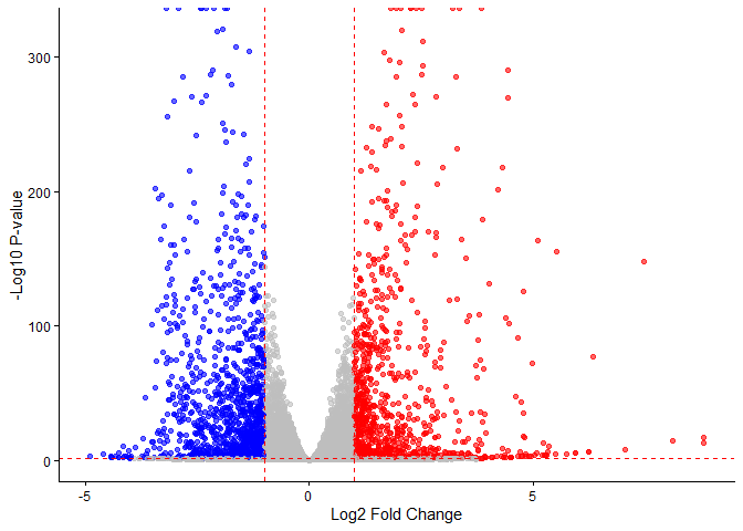
Q4. Improve this plot by completing the below code, which adds color and axis labels
my_cols <- rep("gray", nrow(res))
my_cols[which(res$padj < 0.05 & res$log2FoldChange > 1)] <- "red"
my_cols[which(res$padj < 0.05 & res$log2FoldChange < -1)] <- "blue"
library(ggplot2)
library(ggrepel)

ggplot(res, aes(x = log2FoldChange, y = -log10(pvalue))) +
  geom_point(col = my_cols, alpha = 0.6) +
  theme_classic() +
  geom_vline(xintercept = c(-1, 1), linetype = "dashed", color = "red") +
  geom_hline(yintercept = -log10(0.05), linetype = "dashed", color = "red") +
  labs(x = "Log2 Fold Change", y = "-Log10 P-value")
Warning: Removed 3833 rows containing missing values or values outside the scale range
(`geom_point()`).
  # Only label significant hits:
  geom_text_repel(
    data = subset(res, padj < 0.05 & abs(log2FoldChange) > 1),
    aes(label = genename),
    size = 3
  )
mapping: label = ~genename
geom_text_repel: parse = FALSE, na.rm = FALSE, box.padding = 0.25, point.padding = 1e-06, min.segment.length = 0.5, arrow = NULL, force = 1, force_pull = 1, max.time = 0.5, max.iter = 10000, max.overlaps = 10, nudge_x = 0, nudge_y = 0, xlim = c(NA, NA), ylim = c(NA, NA), direction = both, seed = NA, verbose = FALSE
stat_identity: na.rm = FALSE
position_identity
Pathway analysis
library(gage)
library(gageData)
foldchanges <- res$log2FoldChange
names(foldchanges) <- res$entrezid
head(foldchanges)
    79501      <NA>      <NA>      <NA>      <NA>    148398
       NA        NA 0.1792571        NA        NA 0.4264571
data(kegg.sets.hs)
keggres = gage(foldchanges, gsets=kegg.sets.hs)
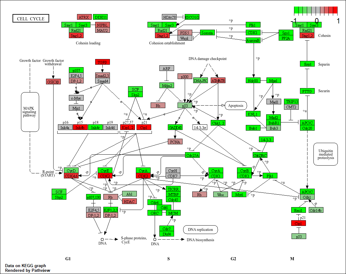
Q5. Can you do the same procedure as above to plot the pathview figures for the top 5 down-reguled pathways?
head(keggres$less,5)
                                                  p.geomean stat.mean
hsa04110 Cell cycle                            7.077982e-06 -4.432593
hsa03030 DNA replication                       9.424076e-05 -3.951803
hsa05130 Pathogenic Escherichia coli infection 1.076420e-04 -3.835716
hsa03013 RNA transport                         1.048017e-03 -3.112129
hsa04114 Oocyte meiosis                        2.563806e-03 -2.827297
                                                      p.val       q.val
hsa04110 Cell cycle                            7.077982e-06 0.001507610
hsa03030 DNA replication                       9.424076e-05 0.007642585
hsa05130 Pathogenic Escherichia coli infection 1.076420e-04 0.007642585
hsa03013 RNA transport                         1.048017e-03 0.055806908
hsa04114 Oocyte meiosis                        2.563806e-03 0.108869849
                                               set.size         exp1
hsa04110 Cell cycle                                 124 7.077982e-06
hsa03030 DNA replication                             36 9.424076e-05
hsa05130 Pathogenic Escherichia coli infection       55 1.076420e-04
hsa03013 RNA transport                              149 1.048017e-03
hsa04114 Oocyte meiosis                             112 2.563806e-03
library(pathview)
##############################################################################
Pathview is an open source software package distributed under GNU General
Public License version 3 (GPLv3). Details of GPLv3 is available at
http://www.gnu.org/licenses/gpl-3.0.html. Particullary, users are required to
formally cite the original Pathview paper (not just mention it) in publications
or products. For details, do citation("pathview") within R.

The pathview downloads and uses KEGG data. Non-academic uses may require a KEGG
license agreement (details at http://www.kegg.jp/kegg/legal.html).
##############################################################################
pathview(gene.data=foldchanges, pathway.id="hsa04110")
'select()' returned 1:1 mapping between keys and columns

Info: Working in directory C:/Users/kavan/Desktop/bggn213_f25_github/Class 13

Info: Writing image file hsa04110.pathview.png
 ### GO Analysis
Let’s try GO analysis and compare to KEGG analysis
data(go.sets.hs)
data(go.subs.hs)

gobpsets = go.sets.hs[go.subs.hs$BP]
gobpres = gage(foldchanges, gsets=gobpsets)
head(gobpres$less, 5)
                                            p.geomean stat.mean        p.val
GO:0048285 organelle fission             6.386337e-16 -8.175381 6.386337e-16
GO:0000280 nuclear division              1.726380e-15 -8.056666 1.726380e-15
GO:0007067 mitosis                       1.726380e-15 -8.056666 1.726380e-15
GO:0000087 M phase of mitotic cell cycle 4.593581e-15 -7.919909 4.593581e-15
GO:0007059 chromosome segregation        9.576332e-12 -6.994852 9.576332e-12
                                                q.val set.size         exp1
GO:0048285 organelle fission             2.515911e-12      386 6.386337e-16
GO:0000280 nuclear division              2.515911e-12      362 1.726380e-15
GO:0007067 mitosis                       2.515911e-12      362 1.726380e-15
GO:0000087 M phase of mitotic cell cycle 5.020784e-12      373 4.593581e-15
GO:0007059 chromosome segregation        8.373545e-09      146 9.576332e-12
Reactome
Some folks really like Reactome online (i.e. their webpage viewer) rather than the R package of the same name (available from Bioconductor).
To use the website viewer we want to upload our set of gene symbols for the genes we want to focus on.
sig_genes <- res$symbol[which(res$padj < 0.05 & !is.na(res$padj))]

write.table(sig_genes, file="significant_genes.txt",
            row.names=FALSE, col.names=FALSE, quote=FALSE)
Q6. What pathway has the most significant “Entities p-value”? Do the most significant pathways listed match your previous KEGG results? What factors could cause differences between the two methods?
“Organelle fission” has the most significant value, where it was cell cycle before. Differences between KEGG and Reactome pathway analysis results can arise from variations in pathway definitions, gene set composition, statistical methods, and biological context considered by each database.
Save results
write.csv(as.data.frame(res), file="DESeq2_results_annotated.csv")
save(res, counts, metadata, file="DESeq2_results_annotated.RData")