Kavi's BGGN 213 Portfolio

Class work for bioinformatics class
Class 19
Kavi Gonur (PID: A69046927)
- Background
- The CMI-PB Project
- Focus in IgG
- Time course of PT (Virulence Factor: Pertussis Toxin)
- System setup
Background
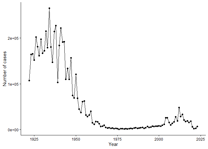
Pertussis (a.k.a Whooping Cough) is a highly infectious lung infection caused by the bacteia B. pertussis.
The CDC tracks case numbers in the US and makes this data available online:
Q1. With the help of the R “addin” package datapasta assign the CDC pertussis case number data to a data frame called cdc and use ggplot to make a plot of cases numbers over time.
library(ggplot2)

cdcgraph <- ggplot(cdc) +
  aes(year, cases) +
  geom_point() +
  geom_line() +
  labs(x="Year",y="Number of cases") +
  theme_classic()

cdcgraph
Q2. Using the ggplot
geom_vline()function add lines to your previous plot for the 1946 introduction of the wP vaccine and the 1996 switch to aP vaccine (see example in the hint below). What do you notice?
cdcgraph +
  geom_vline(xintercept = 1946, linetype="dashed", color = "blue") +
  geom_vline(xintercept = 1996, linetype="dashed", color = "red") +
  geom_vline(xintercept = 2020, linetype="dashed", color = "grey") +
  geom_text(aes(x=1946, y=250000, label="wP"),
            angle=90, vjust = -0.5, color="blue") +
  geom_text(aes(x=1996, y=250000, label="aP"),
            angle=90, vjust = -0.5, color="red")
Warning in geom_text(aes(x = 1946, y = 250000, label = "wP"), angle = 90, : All aesthetics have length 1, but the data has 102 rows.
ℹ Please consider using `annotate()` or provide this layer with data containing
  a single row.

Warning in geom_text(aes(x = 1996, y = 250000, label = "aP"), angle = 90, : All aesthetics have length 1, but the data has 102 rows.
ℹ Please consider using `annotate()` or provide this layer with data containing
  a single row.
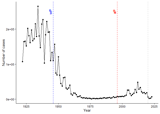
Q3. Describe what happened after the introduction of the aP vaccine? Do you have a possible explanation for the observed trend?
Maybe the vaccine wasn’t as effective as hoped, or there were changes in vaccination rates, pathogen evolution, or reporting practices. Further investigation would be needed to determine the exact cause.
The CMI-PB Project
The CMI-PB project is a collaboration between researchers at UCSD and the Scripps Institution of Oceanography to study the microbial communities in the coastal waters of Southern California. The project involves collecting water samples from various locations along the coast and analyzing the microbial DNA using high-throughput sequencing techniques.
They make their data aavailable via a JSON format running API. E=We can
read JSON format with the read_json function from the jsonlite R
package..
library(jsonlite)
Warning: package 'jsonlite' was built under R version 4.5.2
subject <- read_json("https://www.cmi-pb.org/api/subject", simplifyVector = TRUE)
head(subject, 3)
  subject_id infancy_vac biological_sex              ethnicity  race
1          1          wP         Female Not Hispanic or Latino White
2          2          wP         Female Not Hispanic or Latino White
3          3          wP         Female                Unknown White
  year_of_birth date_of_boost      dataset
1    1986-01-01    2016-09-12 2020_dataset
2    1968-01-01    2019-01-28 2020_dataset
3    1983-01-01    2016-10-10 2020_dataset
Q4. How many aP and wP infancy vaccinated subjects are in the dataset?
table(subject$infancy_vac)
aP wP
87 85
subject$infancy_vac
  [1] "wP" "wP" "wP" "wP" "wP" "wP" "wP" "wP" "aP" "wP" "wP" "wP" "aP" "wP" "wP"
 [16] "wP" "wP" "aP" "wP" "wP" "wP" "wP" "wP" "wP" "wP" "wP" "aP" "wP" "aP" "wP"
 [31] "wP" "aP" "wP" "wP" "wP" "aP" "aP" "aP" "wP" "wP" "wP" "aP" "aP" "aP" "aP"
 [46] "aP" "aP" "aP" "aP" "aP" "aP" "aP" "aP" "aP" "aP" "aP" "aP" "aP" "aP" "aP"
 [61] "wP" "wP" "wP" "wP" "wP" "wP" "wP" "wP" "wP" "aP" "aP" "wP" "wP" "wP" "aP"
 [76] "aP" "wP" "wP" "wP" "wP" "wP" "aP" "aP" "aP" "aP" "aP" "aP" "aP" "aP" "aP"
 [91] "aP" "aP" "aP" "aP" "aP" "aP" "wP" "wP" "aP" "aP" "aP" "aP" "wP" "wP" "wP"
[106] "aP" "aP" "wP" "wP" "aP" "wP" "aP" "aP" "wP" "aP" "aP" "aP" "aP" "aP" "wP"
[121] "aP" "aP" "wP" "aP" "wP" "wP" "aP" "wP" "wP" "wP" "aP" "wP" "aP" "wP" "wP"
[136] "wP" "aP" "aP" "wP" "aP" "wP" "aP" "aP" "aP" "aP" "wP" "aP" "wP" "wP" "wP"
[151] "wP" "wP" "aP" "aP" "aP" "aP" "aP" "aP" "wP" "aP" "aP" "aP" "wP" "wP" "wP"
[166] "aP" "aP" "wP" "aP" "wP" "wP" "wP"
Q5. How many Male and Female subjects/patients are in the dataset?
table(subject$biological_sex)
Female   Male
   112     60
Q6. What is the breakdown of race and biological sex (e.g. number of Asian females, White males etc…)?
table(subject$race, subject$biological_sex)
                                            Female Male
  American Indian/Alaska Native                  0    1
  Asian                                         32   12
  Black or African American                      2    3
  More Than One Race                            15    4
  Native Hawaiian or Other Pacific Islander      1    1
  Unknown or Not Reported                       14    7
  White                                         48   32
Let’s read more tables
library(jsonlite)
specimen <- read_json("https://www.cmi-pb.org/api/v5_1/specimen", simplifyVector = TRUE)
ab_titer <- read_json("https://www.cmi-pb.org/api/v5_1/plasma_ab_titer",simplifyVector = TRUE)
Working with Dates
Q7. Using this approach determine (i) the average age of wP individuals, (ii) the average age of aP individuals; and (iii) are they significantly different?
library(lubridate)
Warning: package 'lubridate' was built under R version 4.5.2


Attaching package: 'lubridate'

The following objects are masked from 'package:base':

    date, intersect, setdiff, union
library(dplyr)
Attaching package: 'dplyr'

The following objects are masked from 'package:stats':

    filter, lag

The following objects are masked from 'package:base':

    intersect, setdiff, setequal, union
subject$age <- today() - ymd(subject$year_of_birth)

# (i)
ap <- subject %>% filter(infancy_vac == "aP")
round(summary(time_length(ap$age, "years" )))
   Min. 1st Qu.  Median    Mean 3rd Qu.    Max.
     23      27      28      28      29      35
 # (ii)
wp <- subject %>% filter(infancy_vac == "wP")
round(summary(time_length(wp$age, "years")))
   Min. 1st Qu.  Median    Mean 3rd Qu.    Max.
     23      33      35      37      40      58
# (iii)
t.test(ap$age,wp$age)
    Welch Two Sample t-test

data:  ap$age and wp$age
t = -12.918 days, df = 104.03, p-value < 2.2e-16
alternative hypothesis: true difference in means is not equal to 0
95 percent confidence interval:
 -3686.855 days -2705.535 days
sample estimates:
Time differences in days
mean of x mean of y
 10165.28  13361.47
1) 28 2) 37 3) yes, significantly different (p 2.2e-16)
Q8. Determine the age of all individuals at time of boost?
subject$boost_age <- ymd(subject$date_of_boost) - ymd(subject$year_of_birth)
round(head(time_length(subject$boost_age,"years")))
[1] 31 51 34 29 26 29
round(summary(time_length(subject$boost_age,"years")))
   Min. 1st Qu.  Median    Mean 3rd Qu.    Max.
     19      21      26      26      30      51
Q9a. With the help of a faceted boxplot or histogram, do you think these two groups are significantly different?
ggplot(subject) +
  aes(time_length(age, "year"),
      fill=as.factor(infancy_vac)) +
  geom_histogram(show.legend=FALSE) +
  facet_wrap(vars(infancy_vac), nrow=2) +
  xlab("Age in years")
`stat_bin()` using `bins = 30`. Pick better value `binwidth`.
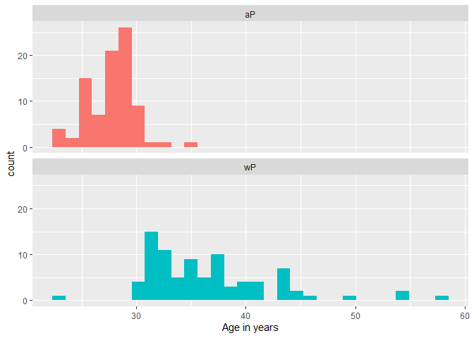
I think they are significantly different!
Join (or link, or merge) using the
Q9b. Complete the code to join specimen and subject tables to make a new merged data frame containing all specimen records along with their associated subject details: Q10. Now using the same procedure join meta with titer data so we can further analyze this data in terms of time of visit aP/wP, male/female etc.
library(dplyr)

meta <- inner_join(subject, specimen)
Joining with `by = join_by(subject_id)`
head(meta)
  subject_id infancy_vac biological_sex              ethnicity  race
1          1          wP         Female Not Hispanic or Latino White
2          1          wP         Female Not Hispanic or Latino White
3          1          wP         Female Not Hispanic or Latino White
4          1          wP         Female Not Hispanic or Latino White
5          1          wP         Female Not Hispanic or Latino White
6          1          wP         Female Not Hispanic or Latino White
  year_of_birth date_of_boost      dataset        age  boost_age specimen_id
1    1986-01-01    2016-09-12 2020_dataset 14586 days 11212 days           1
2    1986-01-01    2016-09-12 2020_dataset 14586 days 11212 days           2
3    1986-01-01    2016-09-12 2020_dataset 14586 days 11212 days           3
4    1986-01-01    2016-09-12 2020_dataset 14586 days 11212 days           4
5    1986-01-01    2016-09-12 2020_dataset 14586 days 11212 days           5
6    1986-01-01    2016-09-12 2020_dataset 14586 days 11212 days           6
  actual_day_relative_to_boost planned_day_relative_to_boost specimen_type
1                           -3                             0         Blood
2                            1                             1         Blood
3                            3                             3         Blood
4                            7                             7         Blood
5                           11                            14         Blood
6                           32                            30         Blood
  visit
1     1
2     2
3     3
4     4
5     5
6     6
ab_data <- inner_join(meta,ab_titer)
Joining with `by = join_by(specimen_id)`
head(ab_data)
  subject_id infancy_vac biological_sex              ethnicity  race
1          1          wP         Female Not Hispanic or Latino White
2          1          wP         Female Not Hispanic or Latino White
3          1          wP         Female Not Hispanic or Latino White
4          1          wP         Female Not Hispanic or Latino White
5          1          wP         Female Not Hispanic or Latino White
6          1          wP         Female Not Hispanic or Latino White
  year_of_birth date_of_boost      dataset        age  boost_age specimen_id
1    1986-01-01    2016-09-12 2020_dataset 14586 days 11212 days           1
2    1986-01-01    2016-09-12 2020_dataset 14586 days 11212 days           1
3    1986-01-01    2016-09-12 2020_dataset 14586 days 11212 days           1
4    1986-01-01    2016-09-12 2020_dataset 14586 days 11212 days           1
5    1986-01-01    2016-09-12 2020_dataset 14586 days 11212 days           1
6    1986-01-01    2016-09-12 2020_dataset 14586 days 11212 days           1
  actual_day_relative_to_boost planned_day_relative_to_boost specimen_type
1                           -3                             0         Blood
2                           -3                             0         Blood
3                           -3                             0         Blood
4                           -3                             0         Blood
5                           -3                             0         Blood
6                           -3                             0         Blood
  visit isotype is_antigen_specific antigen        MFI MFI_normalised  unit
1     1     IgE               FALSE   Total 1110.21154       2.493425 UG/ML
2     1     IgE               FALSE   Total 2708.91616       2.493425 IU/ML
3     1     IgG                TRUE      PT   68.56614       3.736992 IU/ML
4     1     IgG                TRUE     PRN  332.12718       2.602350 IU/ML
5     1     IgG                TRUE     FHA 1887.12263      34.050956 IU/ML
6     1     IgE                TRUE     ACT    0.10000       1.000000 IU/ML
  lower_limit_of_detection
1                 2.096133
2                29.170000
3                 0.530000
4                 6.205949
5                 4.679535
6                 2.816431
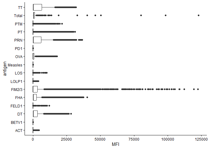
Q11. How many specimens (i.e. entries in abdata) do we have for each isotype?
head(ab_data$isotype)
[1] "IgE" "IgE" "IgG" "IgG" "IgG" "IgE"
How many different antigens are there in the dataset?
unique(ab_data$antigen)
 [1] "Total"   "PT"      "PRN"     "FHA"     "ACT"     "LOS"     "FELD1"
 [8] "BETV1"   "LOLP1"   "Measles" "PTM"     "FIM2/3"  "TT"      "DT"
[15] "OVA"     "PD1"
ggplot(ab_data) +
  aes(MFI,antigen) +
  geom_boxplot() +
  theme_classic()
Warning: Removed 1 row containing non-finite outside the scale range
(`stat_boxplot()`).
Q12. What are the different $dataset values in abdata and what do you notice about the number of rows for the most “recent” dataset?
table(ab_data$dataset)
2020_dataset 2021_dataset 2022_dataset 2023_dataset
       31520         8085         7301        15050
There’s a lot more rows in the most recent dataset!
Focus in IgG
IgG is crucial for long-term immunity and responding to bacterial and viral infections
ab_data |>
  filter(isotype == "IgG") -> igg_data
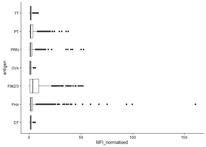
Plot of antigen levels again but for IgG only
igg_dataplot <- ggplot(igg_data) +
  aes(x=MFI_normalised, y=antigen) +
  geom_boxplot() +
  theme_classic()
igg_dataplot
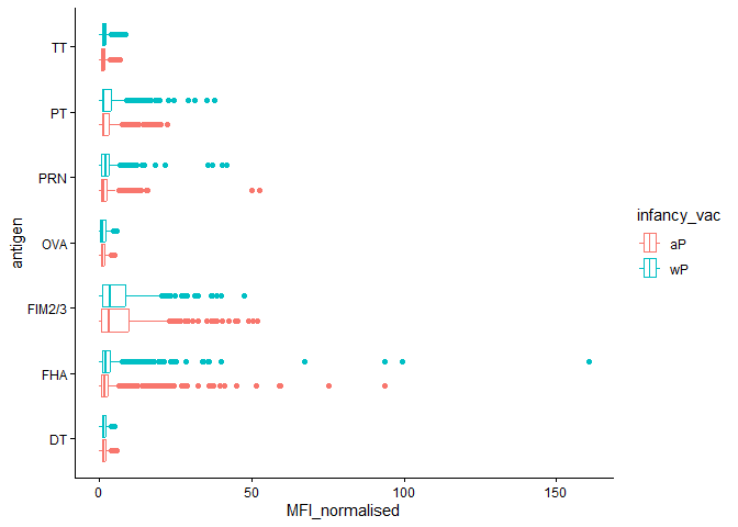
Differences between aP and wP?
We can color up by the infancy_vac values of “wP” or “aP”
igg_dataplot +
  aes(color=infancy_vac)
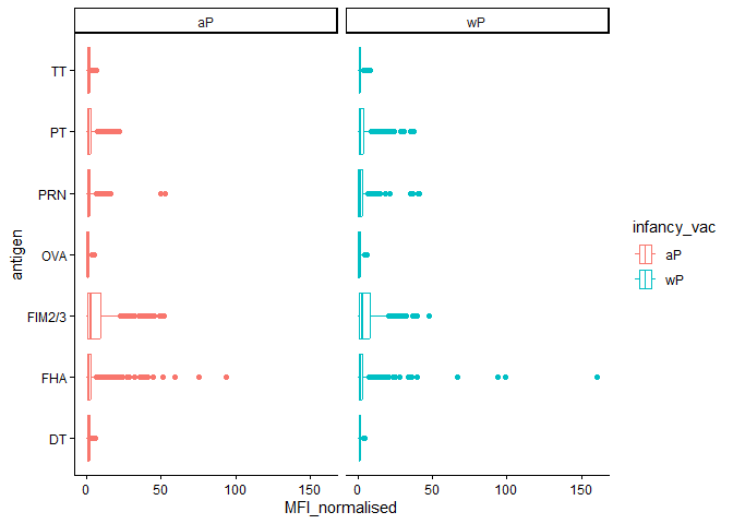
We could “facet” by the “aP” vs “wP” column
igg_dataplot +
  aes(color=infancy_vac) +
  facet_wrap(~infancy_vac)
Time course analysis
Q13. Complete the following code to make a summary boxplot of Ab titer levels (MFI) for all antigens:
We can use visit as a proxy for time here and facet our plots by this
value 1 to 8…
igg_data |>
  filter(visit %in% 1:8) |>
  ggplot() +
    aes(x=MFI_normalised,y=antigen,color=infancy_vac) +
    facet_wrap(~visit) +
    geom_boxplot() +
    theme_classic()
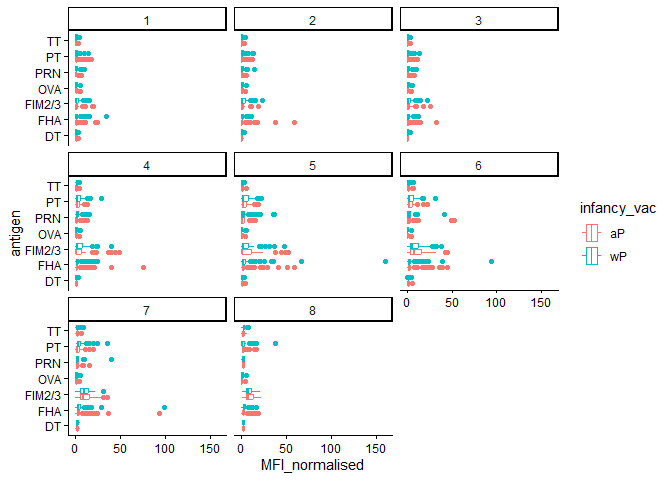
Q14. What antigens show differences in the level of IgG antibody titers recognizing them over time? Why these and not others?
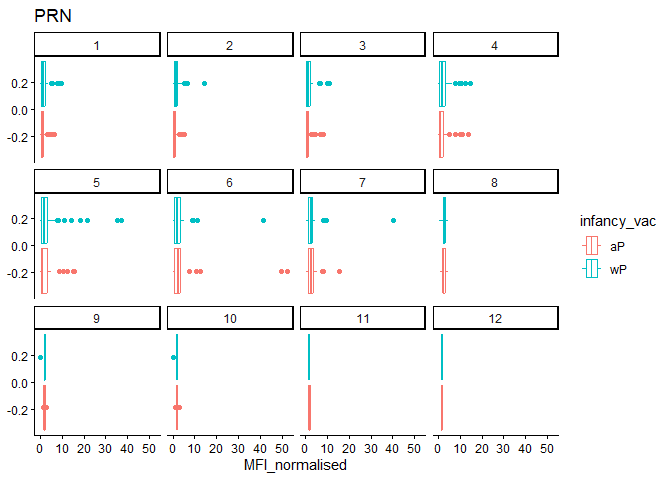
Q15. Filter to pull out only two specific antigens for analysis and create a boxplot for each. You can chose any you like. Below I picked a “control” antigen (“OVA”, that is not in our vaccines) and a clear antigen of interest (“PT”, Pertussis Toxin, one of the key virulence factors produced by the bacterium B. pertussis).
library(dplyr)
filter(igg_data, antigen=="PRN") %>%
  ggplot() +
  aes(MFI_normalised, col=infancy_vac) +
  geom_boxplot(show.legend = TRUE) +
  facet_wrap(vars(visit)) +
  theme_classic() +
  labs(title="PRN")
filter(igg_data, antigen=="FIM2/3") %>%
  ggplot() +
  aes(MFI_normalised, col=infancy_vac) +
  geom_boxplot(show.legend = TRUE) +
  facet_wrap(vars(visit)) +
  theme_classic() +
  labs(title="FIM2/3")
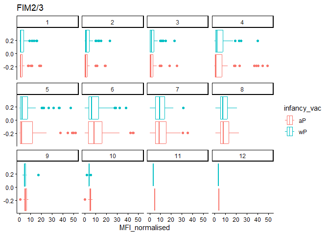
Q16. What do you notice about these two antigens time courses and the PT data in particular?
Of the data presented in the example: PT levels overtime rise and exceed OVA. In this dataset, FIM levels start out large but drop significantly more than PRN (this could be becuse FIM just had a greater range of values than PRN.)
Q17. Do you see any clear difference in aP vs. wP responses?
PRN: Responses about the same FIM: For most part, aP > wP.
Time course of PT (Virulence Factor: Pertussis Toxin)
(removed dataset displays here, made rendering take WAYYYY too long)
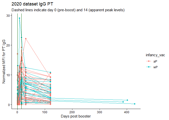
pt_2020 <- igg_data |>
  filter(antigen == "PT") |>
  filter(dataset == "2020_dataset")
pt_2021 <- igg_data |>
  filter(antigen == "PT") |>
  filter(dataset == "2021_dataset")
pt_2020 |>
  ggplot() +
    aes(planned_day_relative_to_boost,
        MFI_normalised,
        color=infancy_vac,
        group=subject_id) +
    geom_point() +
    geom_line() +
    theme_classic() +
    geom_vline(xintercept=0, col="darkgreen") +
    geom_vline(xintercept =14, col="darkgreen") +
    labs(title="2020 dataset IgG PT",
       subtitle = "Dashed lines indicate day 0 (pre-boost) and 14 (apparent peak levels)",x="Days post booster", y="Normalized MFI for PT IgG")
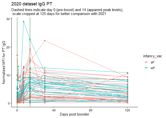
pt_2020 |>
  ggplot() +
    aes(planned_day_relative_to_boost,
        MFI_normalised,
        color=infancy_vac,
        group=subject_id) +
    geom_point() +
    geom_line() +
    theme_classic() +
    geom_vline(xintercept=0, col="darkgreen") +
    geom_vline(xintercept =14, col="darkgreen") +
    scale_x_continuous(limits = c(0, 125)) +
    labs(title="2020 dataset IgG PT",
       subtitle = "Dashed lines indicate day 0 (pre-boost) and 14 (apparent peak levels), \n scale cropped at 125 days for better comparison with 2021",x="Days post booster", y="Normalized MFI for PT IgG")
Warning: Removed 3 rows containing missing values or values outside the scale range
(`geom_point()`).

Warning: Removed 3 rows containing missing values or values outside the scale range
(`geom_line()`).
pt_2021 |>
  ggplot() +
    aes(planned_day_relative_to_boost,
        MFI_normalised,
        color=infancy_vac,
        group=subject_id) +
    geom_point() +
    geom_line() +
    theme_classic() +
    geom_vline(xintercept=0, col="darkgreen") +
    geom_vline(xintercept =14, col="darkgreen") +
    labs(title="2021 dataset IgG PT",
       subtitle = "Dashed lines indicate day 0 (pre-boost) and 14 (apparent peak levels)",x="Days post booster", y="Normalized MFI for PT IgG")
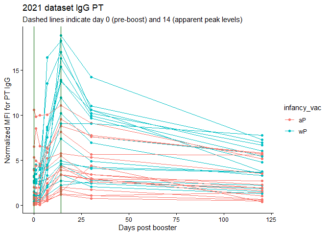
Q18. Does this trend look similar for the 2020 dataset?
Hard to tell - the 2020 trend looks quite smushed bnecause of twice the number of days being recorded. I would guess probably.
Actually, no, MFIs were HIGHER in 2020 at 14 days.
System setup
sessionInfo()
R version 4.5.1 (2025-06-13 ucrt)
Platform: x86_64-w64-mingw32/x64
Running under: Windows 11 x64 (build 26200)

Matrix products: default
  LAPACK version 3.12.1

locale:
[1] LC_COLLATE=English_United States.utf8
[2] LC_CTYPE=English_United States.utf8
[3] LC_MONETARY=English_United States.utf8
[4] LC_NUMERIC=C
[5] LC_TIME=English_United States.utf8

time zone: America/Los_Angeles
tzcode source: internal

attached base packages:
[1] stats     graphics  grDevices utils     datasets  methods   base

other attached packages:
[1] dplyr_1.1.4     lubridate_1.9.4 jsonlite_2.0.0  ggplot2_4.0.0

loaded via a namespace (and not attached):
 [1] vctrs_0.6.5        cli_3.6.5          knitr_1.50         rlang_1.1.6
 [5] xfun_0.53          generics_0.1.4     S7_0.2.0           labeling_0.4.3
 [9] glue_1.8.0         htmltools_0.5.8.1  scales_1.4.0       rmarkdown_2.30
[13] grid_4.5.1         evaluate_1.0.5     tibble_3.3.0       fastmap_1.2.0
[17] yaml_2.3.10        lifecycle_1.0.4    compiler_4.5.1     RColorBrewer_1.1-3
[21] timechange_0.3.0   pkgconfig_2.0.3    rstudioapi_0.17.1  farver_2.1.2
[25] digest_0.6.37      R6_2.6.1           tidyselect_1.2.1   pillar_1.11.1
[29] magrittr_2.0.4     withr_3.0.2        tools_4.5.1        gtable_0.3.6